고정 헤더 영역
상세 컨텐츠
본문
728x90
정제한 데이터에 필지 별로 거점을 부여한다. 정확히는 행위자가 이용할 것으로 예상되는 거점을 matching 한다. 17개 거점 중 행위자가 어떤 거점을 이용할까. 당연히 제일 가까운 곳을 이용할 가능성이 크다. 해서, 행위자 기준 100m 이내에 위치한 거점을 대상 거점으로 부여했다. 100m 이내에 거점이 없는 행위자는 150m 이내 가장 가까운 거점 한 곳을 부여했다.
#%% New Point 좌표 생성
new_point = {'point_number':range(0, 17),
              'geometry':[Point(197386.30,442712.87), Point(197538.45,442701.02), Point(197443.36,442582.25), Point(197398.14,442500.79), Point(197847.41,442528.07),
                    Point(197546.34,442469.94), Point(197669.78,442467.06), Point(197737.24,442488.59), Point(197264.30,442434.05), Point(197270.76,442360.13),
                    Point(197440.13,442383.82), Point(197601.60,442335.01), Point(197519.07,442228.80), Point(197427.21,442180.00), Point(197380.56,442071.63),
                    Point(197326.74,442041.49), Point(197308.80,442511.56)]}

new_point = gpd.GeoDataFrame(new_point, geometry='geometry')
new_point = new_point.set_crs(epsg=5181, inplace=True)

new_point.to_file(save_dir + '/New Point/new_point.shp', encoding='cp949')


#%% 거리 연산
sd = gpd.read_file(save_dir + '/sadang4/sadang4.shp', encoding='cp949')
new_point = gpd.read_file(save_dir + '/New Point/new_point.shp', encoding='cp949')


def shortest_distance_func(df1, df2):
    nearest_point = []

    for t in tqdm(df1['geometry'], leave=True):
        point = []

        for idx, n in enumerate(df2['geometry']):
            d = t.distance(n)

            if d <= 100:
                point.append(idx)


        if len(point) == 0:
            for idx, n in enumerate(df2['geometry']):
                if t.distance(n) <= 150:
                    point.append(idx)

        nearest_point.append(point)

    return nearest_point


near_point = shortest_distance_func(sd, new_point)
sd['near_point'] = near_point

sd = sd[['PNU', 'JIBUN', 'PPK', 'USE_CODE_0', 'USE_CODE_1', 'SD', 'GG', 'near_point', 'geometry']]

del near_point
이제 데이터 정제가 끝났으니 본격적으로 쓰레기 배출 시뮬레이션 소스코드를 살펴본다. 시뮬레이션 규칙은 다음과 같다.
1. 행위자는 세대로 정한다.
2. 행위자는 1 ~ 7 일 중 랜덤으로 쓰레기 배출 주기를 부여받는다.
3. 쓰레기 배출일이 되면 0 ~ 23 시 중 랜덤으로 쓰레기 배출 시간을 부여받는다.
* 쓰레기 수거는 21 시에 이루어지며, 21 시 이후에 쌓인 쓰레기는 다음날 수거된다.
* 쓰레기 배출 시간은 아래와 같이 시간 별로 가중치를 가진다.
[ 0 1 2 3 4 5 6 7 8 9 10 11 12 13 14 15 16 17 18 19 20 21 22 23 ]
[ 1 1 1 1 1 1 1 1 2 2 2 2 2 2 2 2 2 3 3 3 3 3 2 2 ]
4. 행위자는 쓰레기 배출 시 아래 식에 따른 양만큼의 쓰레기를 배출한다.
(배출량) = (배출 주기) X (사당 4동 평균 세대 별 인구) X (동작구 일별 1인당 평균 쓰레기 배출량)
ex) 3일 만에 쓰레기 배출하는 경우, 3 X 1.94 X 0.8 = 4.656 (kg) 배출
규칙을 알고리즘으로 구현한 코드는 다음과 같다.
def simulation_func(df1, df2, days, waste_type, seed):
    time_weight = np.array([1, 1, 1, 1, 1, 1, 1, 1, 2, 2, 2, 2, 2, 2, 2, 2, 2, 3, 3, 3, 3, 3, 3, 2])
    wt = {'일반':1.98*0.8*0.361, '재활용':1.98*0.8*0.361, '음식물':1.98*0.8*0.278}

    random.seed(seed)

    result = np.zeros((days, len(df2)))

    ems_cycle = []                                                             # 배출 주기 생성
    for e in range(len(df1)):
        ems_cycle.append(random.choices(range(1, 7))[0])
    ems_cycle = np.array(ems_cycle)
    ems_cycle_cal = ems_cycle.copy()

    for d in range(days):
        ems_cycle -= 1

        target = np.where(ems_cycle == 0)[0]                                   # 배출 행위자

        ems_time = []                                                          # 행위자 별 배출 시간
        ems_point = []                                                         # 배출 Point
        for ta in target:
            ems_time.append(random.choices(range(0, 24),
                                           weights=time_weight)[0])
            ems_point.append(random.choices(sd['near_point'][ta])[0])
        ems_time = np.array(ems_time)
        ems_point = np.array(ems_point)

        for p in df2['point_numb']:
            t = np.where(ems_point == p)[0]

            for a in t:
                if ems_time[a] <= 21:
                    result[d, p] += df1['SD'][a] * wt[waste_type] * ems_cycle_cal[a]

                elif d < days - 1:
                    result[d, p] += df1['SD'][a] * wt[waste_type] * ems_cycle_cal[a]

        for ta in target:
            ems_cycle[ta] = random.choices(range(1, 7))[0]
            ems_cycle_cal[ta] = random.choices(range(1, 7))[0]

    return pd.DataFrame(result)

waste_general, waste_food, waste_recycle = simulation_func(sd, new_point, 30, '일반', 123), simulation_func(sd, new_point, 30, '음식물', 124), simulation_func(sd, new_point, 30, '재활용', 125)
실제 시뮬레이션에서는 4 번 규칙이 약간 변경되었다. 쓰레기 종류를 구분했다. 평균적으로
[ 음식물 쓰레기 : 일반 쓰레기 : 재활용 쓰레기 = 1 : 1.3 : 1.3 ] 비율로 배출되기 때문에 4.656 (kg) 을 해당 비율로 나눴다.
쓰레기 종류 별로 random seed 값을 다르게 준 이유는 쓰레기 배출을 한꺼번에 하지는 않는다고 생각했기 때문이다. 내가 아는 한, 그때그때 쓰레기통이 꽉 차면 버리는 경우가 많아서 seed 를 다르게 줬다. 아님 말고~ 고치면 된다. 사실 seed 값이 다르다고 해서 결과가 크게 달라지지는 않는다. 행위자 수가 가장 큰 영향을 미치는 모양이다.
시뮬레이션 결과의 기술통계는 다음과 같다.
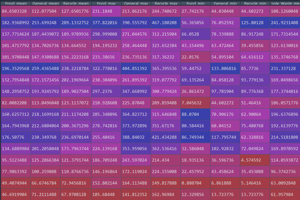

기술 통계량 중 평균치를 기준으로 위계를 설정했다. 하루 150 (kg) 까지는 0, 200 (kg) 까지는 1, 그 이상은 2로 설정하고 mapboxgl 라이브러리를 이용해 맵박스로 나타냈다.
#%% 시각화
# Barplot
plt.figure(figsize = (15, 10))
sns.boxplot(data = waste_general)
plt.title('General_Waste', size = 15)
plt.savefig(save_dir + '/Img/General_Waste.png', dpi=100)
plt.show()

plt.figure(figsize = (15, 10))
sns.boxplot(data = waste_food)
plt.title('Food_Waste', size = 15)
plt.savefig(save_dir + '/Img/Food_Waste.png', dpi=100)
plt.show()

plt.figure(figsize = (15, 10))
sns.boxplot(data = waste_recycle)
plt.title('Recycle_Waste', size = 15)
plt.savefig(save_dir + '/Img/Recycle_Waste.png', dpi=100)
plt.show()

del waste_food, waste_general, waste_recycle, dsc_sts


new_point['geometry'] = new_point.buffer(5)

result = sd[['PNU', 'SD', 'geometry']]
result = pd.concat([result, new_point])
result = result.fillna('-')
result = result.to_crs(epsg=4326)

result.to_file(save_dir + '/Result/Result.shp', encoding='cp949')


# shp -> geojson 변환
sf = shapefile.Reader(save_dir + '/Result/Result')

field_names = ['PNU', 'SD', 'point_numb', 'hierachy']

fields = sf.fields[1:]
for idx, field in enumerate(fields):
    field[0] = field_names[idx]

del idx, field

geometry = []
for sr in sf.shapeRecords():
    atr = dict(zip(field_names, sr.record))

    geom = sr.shape.__geo_interface__
    geometry.append(dict(type="Feature", geometry=geom, properties=atr))

geojson = open(save_dir + '/Result/Result.geojson', "w")
geojson.write(json.dumps({"type": "FeatureCollection", "features": geometry}, indent=2, ensure_ascii=False))
geojson.close()


# Mapbox 시각화
geo_data = save_dir + '/Result/Result.geojson'

with open(geo_data) as f:
    data = json.loads(f.read())

token = 'pk.eyJ1IjoiZ2xvd2Z1ciIsImEiOiJjbDhpYXY4dzIwcDFxM3htcm4zcTZvNW5yIn0.BkTWPUipoFZZoCeifngJiw'
# 이건 내 토큰이니까 각자 발급해서 쓰세용
center = [126.9716483,37.4809714]

match_color_stops = [
    ['0', 'rgb(255,255,0)'],
    ['1', 'rgb(255,165,0)'],
    ['2', 'rgb(255,69,0)']]
match_height_stops = [
    ['0', 10],
    ['1', 10],
    ['2', 10]]

viz = ChoroplethViz(
    access_token = token,
    data = data,
    color_function_type = 'match',
    color_property = 'hierachy',
    color_stops = match_color_stops,
    color_default ='rgb(128,128,128)',
    center = center,
    zoom = 16)

viz.bearing = -15
viz.pitch = 45
viz.height_function_type = 'match'
viz.height_property = 'hierachy'
viz.height_stops = match_height_stops


html = open(save_dir + '/Result/Visualization.html', "w", encoding="utf-8")
html.write(viz.create_html())
html.close()
맵박스 시각화 결과는 다음과 같다.
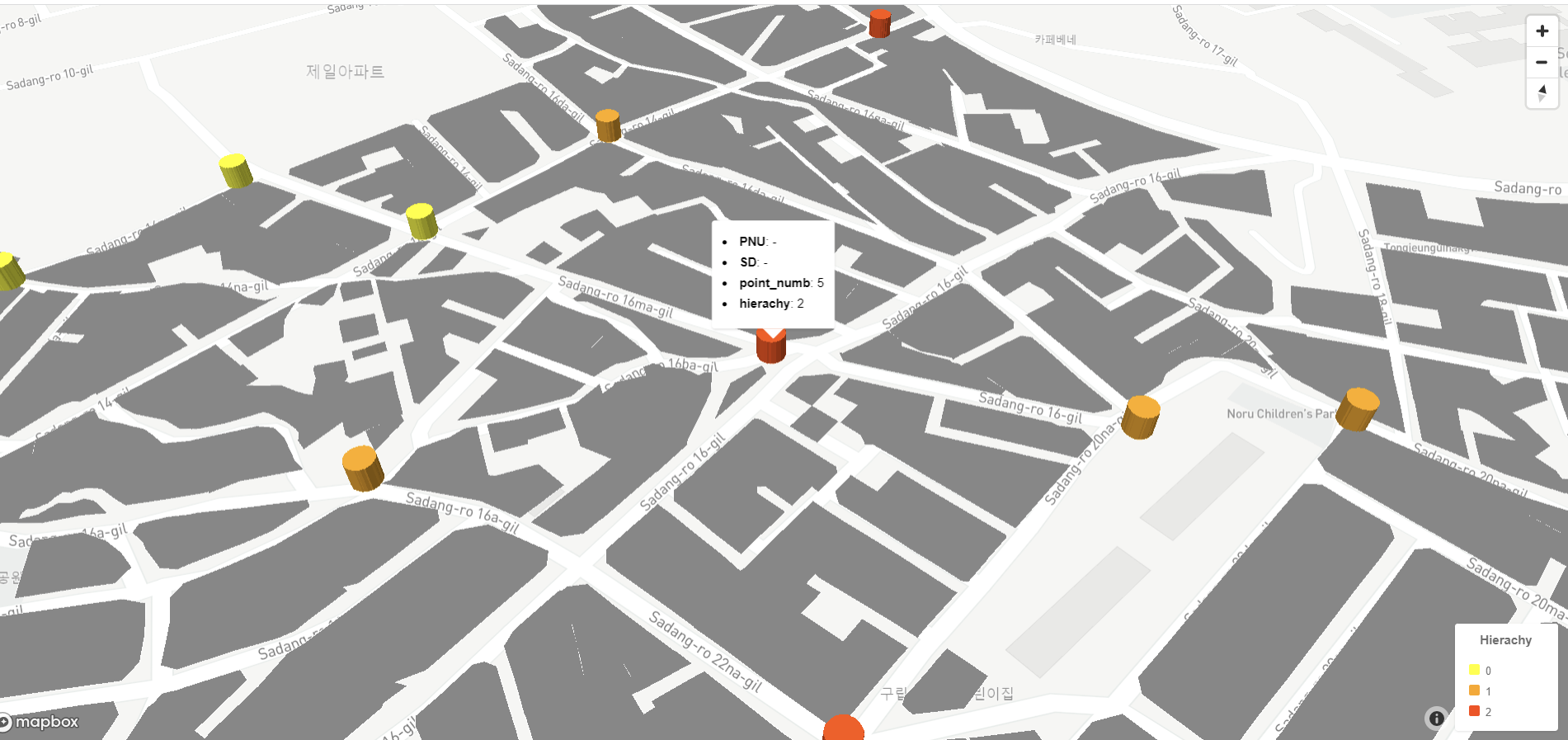
시뮬레이션 결과는 반복 수행에도 크게 변화하지 않았다. 거점 별 수용량이 적절하게 계산되었다고 볼 수 있을 것 같다. 다만, 음식점이나 시장, 편의점 등에서 배출되는 쓰레기 처리 실태를 모르다 보니, 꽤 큰 변수를 제외하고 만들어진 시뮬레이션이라는 점에서 문제가 있다고 생각한다.
시뮬레이션과는 별개로 거점들의 위치가 적절한지, 님비현상을 어떻게 해결할건 지 등 중차대한 문제가 남아있다. 지도 상에서 유휴부지를 걸러내는 알고리즘을 만들어서 거점을 보다 적절하게 배치해 볼 생각이다.
'Algorithm' 카테고리의 다른 글
| [Algorithm] New Point 쓰레기 처리 시스템 구축 알고리즘 (2) Data Preprocessing (0) | 2023.02.19 |
|---|---|
| [Algorithm] New Point 쓰레기 처리 시스템 구축 알고리즘 (1) Project Structure (0) | 2023.02.19 |
| [Algorithm] 쓰레기 배출 시뮬레이션 (1) (0) | 2023.01.09 |
| [Algorithm] 도시화과정 시뮬레이션 (0) | 2023.01.02 |
| [Algorithm] 클러스터링 심화_이미지 처리 1 (2) (0) | 2022.12.25 |


